データの可視化と解析ツール

２次元グラフ: $ plot(x,y,...)

dat=import1("cos.dat");
[n,m]=size(dat);
cx=dat[1:n,1];
cy=dat[1:n,2];
sx=-2*pi:pi/25:2*pi;
plot(sx,sin(sx), "linewidth",2,"linecolor",4, 
     "toplabel", "plot2D", 
     "xlabel", "X-label", "ylabel", "Y-label",
     cx, cy, "linestyle", 0, 
     "markertype", 12, "markersize", 5.0, "markercolor", 3, 
     "-nodate -noxplot -print -colorps -scale 0.7 -o plot2d.ps");
#
# tela -b plaot2d.t
# -noxplot により X11 には何も現れない．
#

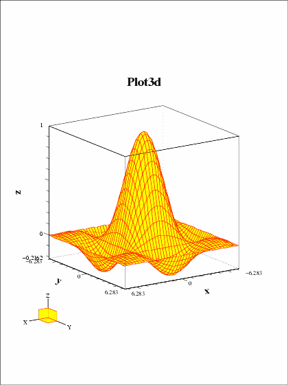
３次元グラフ: $ mesh(z,...)

R=2*pi; dR=0.1*pi;
d=1e-6;
[x,y]=grid(-R-d:dR:R,-R-d:dR:R);
mesh(sin(x)*sin(y)/(x)/(y), "hiddenline", "true",
     "xmin",-R,"xmax",R,"ymin",-R,"ymax",R,
     "toplabel", "Plot3d", "comment", "",
     "-colorps -nodate -scale 0.7 -o plot3d.ps");
#
# tela -b plot3d.t
# で現れた plotMTV の画面で Left Right Up Down などで視点を調整
# Save PS ボタンを押すと 
# plot3d.ps（既定は datplot.ps） が作成される
#

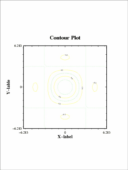
等高線図: contour(z,...)

d=1e-6;
[x,y]=grid(-2*pi-d:0.1*pi:2*pi,-2*pi-d:0.1*pi:2*pi);
contour(sin(x)*sin(y)/(x)/(y),
        "cmin", -0.6, "cmax", 1.0, "nsteps", 8,
        "xmin", -2*pi, "xmax", 2*pi,
        "ymin", -2*pi, "ymax", 2*pi,
        "xlabel", "X-label",
        "ylabel", "Y-lable",
        "toplabel", "Contour Plot", 
        "comment", "",
        "-noxplot -print -nodate -colorps -scale 0.7 -o contour.ps");

２次元グラフ: $ plot(x,y,...)

３次元グラフ: $ mesh(z,...)

等高線図: contour(z,...)

マルチプロット： n/a